We left off the previous episode with some mixed results from combining forward and backward Markov models, but with some promising directions to explore. But before getting to that, I'm forcing myself to do the care and maintenance first.

New eval: Extra words

Another common category of typographical error is the extra word. Either duplicates or a half-completed thought that didn't get fully deleted or a self-correction during dictation, they come up a lot. It will help broaden the set of proofreading errors I expect my proofreader to catch. Also, there weren't enough eval categories to fill up two rows of three plots in the results, and that was bugging me. Now we'll have two full rows.

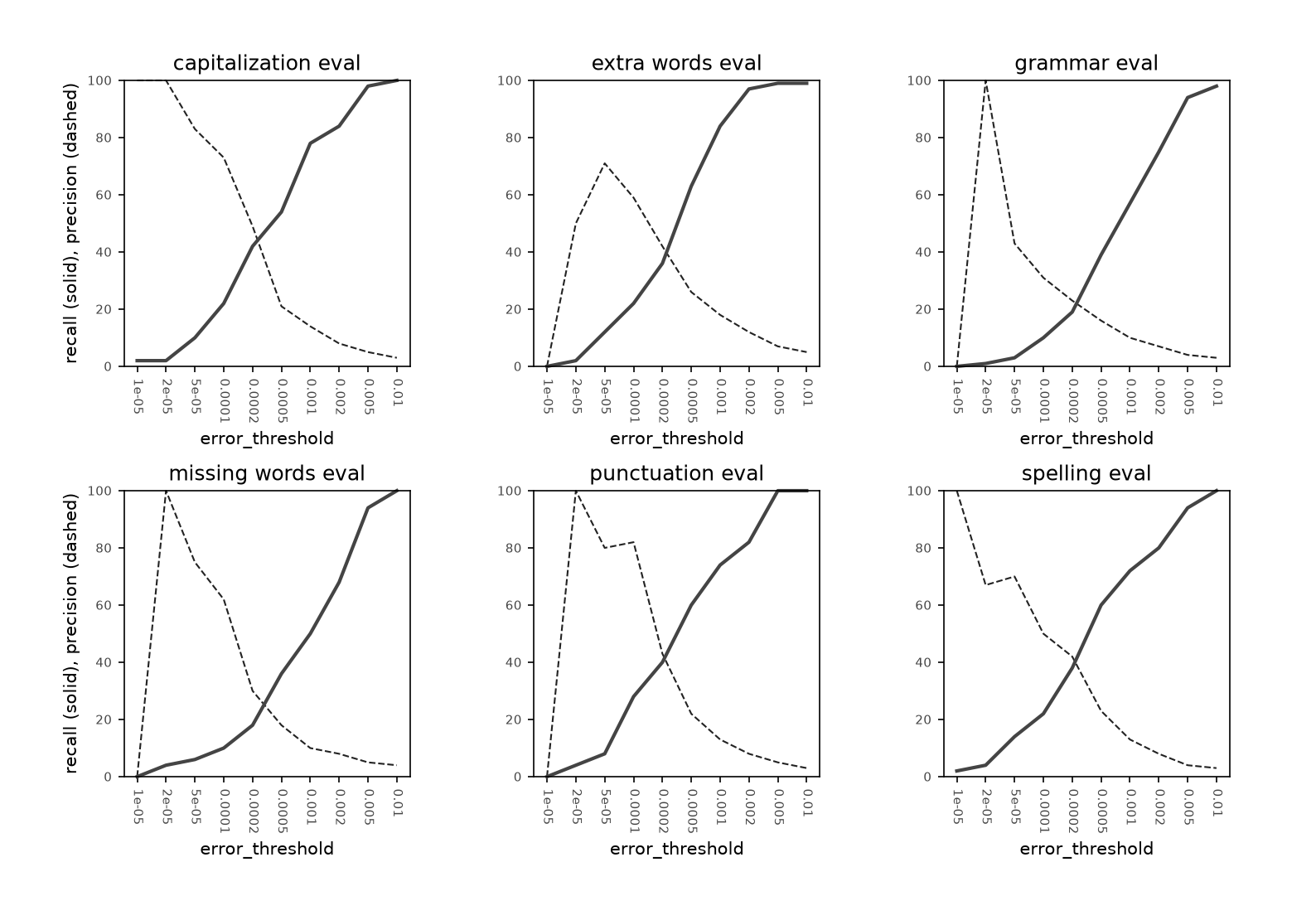
The general form of the extra-word eval matches that of the others. No big revelations here. That in itself is actually forming an interesting pattern. These various categories of errors are all quite different, so the fact that they behave in a roughly similar way is notable. I don't know why that should be the case, but it bodes well for building one model that can detect them all.

New visualization: Precision-recall curve

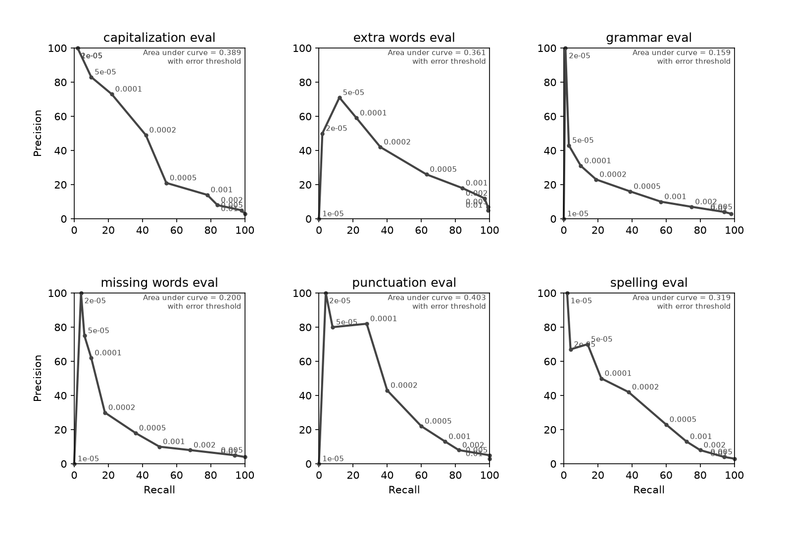
Interpreting the precision and recall plots it tricky because it is the combination of precision-recall pairs that tell the full story. A high precision with a low recall means something very different than when it's paired with a high recall.

A more intuitive way to communicate these coupled relationships is with a precision-recall curve. It is conceptually related to the classic reciever-operator characteristic curve. As with the ROC curve, the area under the PR curve is a convenient metric for the performance of the model. In both cases an area of one represents an ideal model, one that can achieve perfect recall and perfect precision at the same time. Currently the models we're working with range from 0.16 to 0.40 on these evals, so there is room for improvement.

Other ways to combine two models

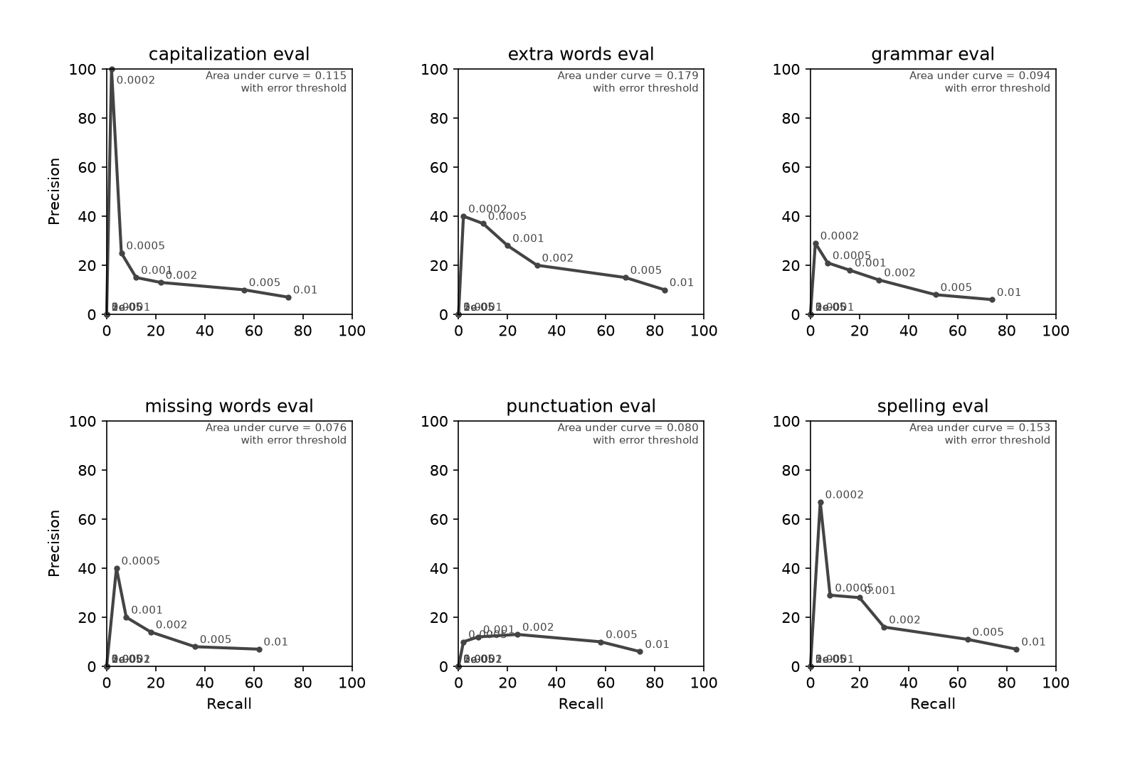
So far we’ve only looked at one way to combine multiple models' estimates, the minimum function. We had good reasons for this, but it’s worthwhile to explore some other options as well. There’s no reason at all to expect the maximum() function to do well. If every model has its own blind spots, then max adds those blind spots altogether, instead of covering them like min does. As expected, the performance is considerably worse. Area under the curve (AUC) varies between 0.08 and 0.18. But it’s still useful as a floor, showing how rough things can get if we go with something that we expect to be wrong.

A weakness of both the min and max functions is that they let any single model cast the deciding vote on whether a particular token is in error. This makes for a brittle system, only as accurate as the flakiest model involved. To build in some resilience it’s useful to combine the models in a way that every vote carries some weight. The most generic way to do this is with the mean() function—straight up add every model's estimate and divide by the number of models.

This too gives kind of a wonky estimate, slightly better than max. AUC range is 0.08 to 0.24.

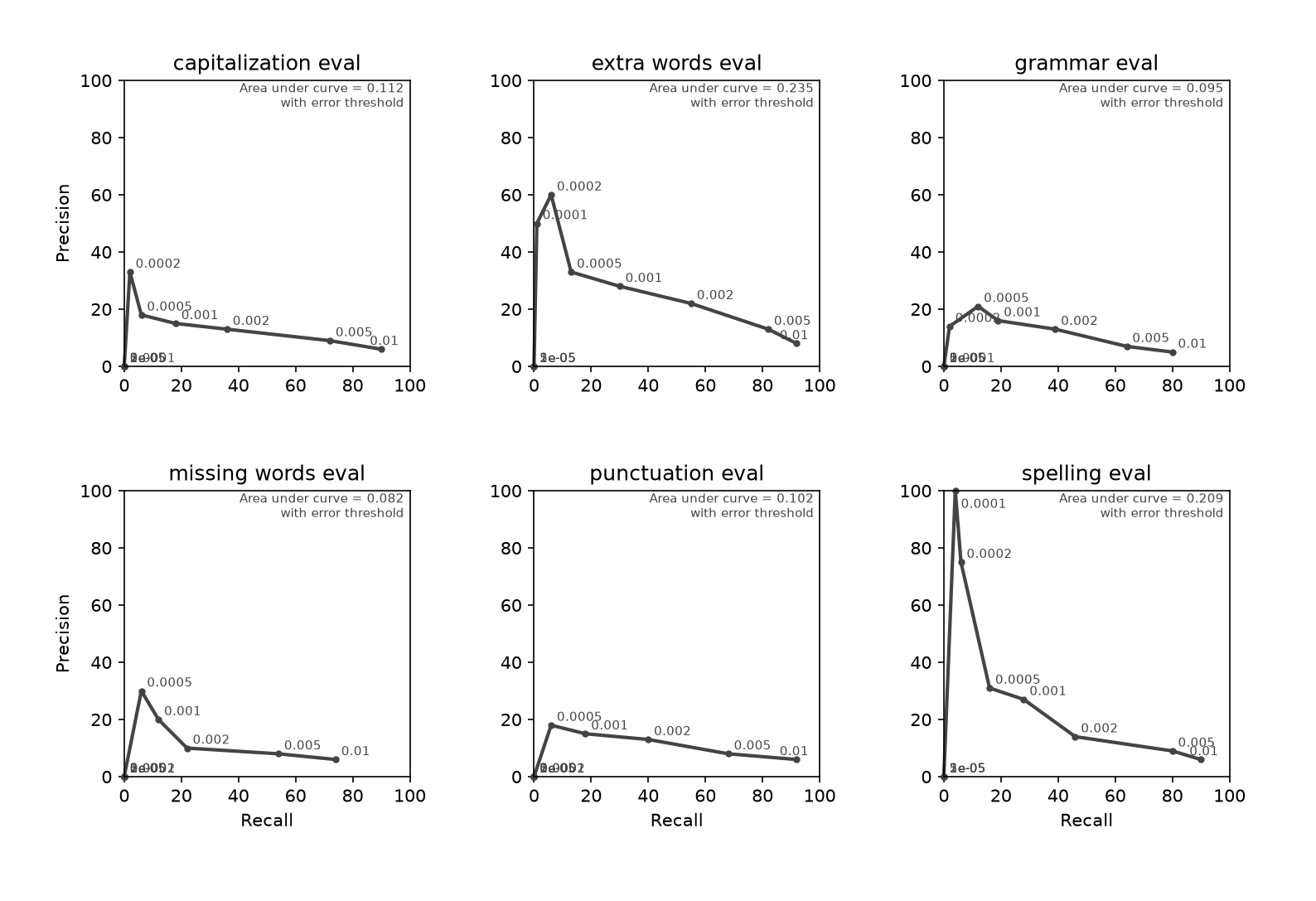
It’s not much better than using the max. That may be because combining small numbers is tricky to do in a meaningful way. Taking the average of 1e-3 (10^-3) and 1e-7 produces something that is halfway in between them, but on a logarithmic scale, it ends up being much closer to 1e-3. A medium-sized likelihood averaged with a very small likelihood ends up looking like a medium-sized likelihood.

To properly account for this, we can use the geometric mean. As opposed to the vanilla mean, a.k.a. the arithmetic mean, the geometric mean multiplies all N elements together, and then takes the N-th root of them. In this case, the geometric mean of 1e-3 and 1e-7 would end up being 1e-5, something that is closer to being in the middle of those two, at least for the our purposes. The geometric mean has a nice property that it gives every model a vote, but it gives extra weight to low likelihood estimates. It falls somewhere in between the minimum winner-take-all estimate and the mean.

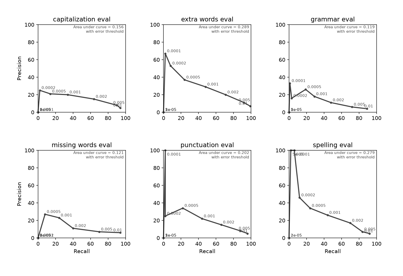
Sadly, despite all of the good reasons we have for thinking this is a brilliant approach, it doesn’t perform much better than the max or the min. AUC range is a lukewarm 0.12 to 0.29, a good bit lower than the min function. In fact a tedious exploration of error thresholds, model alphabet sizes, and β values fails to do much better.

This is a bummer and a good reminder that no matter how good a theory sounds, there’s no guarantee that it will play out in reality the way you picture it going in your head.

Classic additive smoothing, an α parameter

I wasn't ready to give up on the geometric mean yet. The reasons for using it are still valid (less sensitivity to a single rogue model). And it's helpful to remember that the β factor was designed specifically to help the minimum comparison be more meaningful. It way overestimates the likelihoods of tokens until a critical mass of observations have been collected. The success of β for min-based combination suggests that maybe another correction might lead to a performance improvement for geometric mean-based model combination. A reasonable thing to try is the original additive smoothing approach (without an upward bias) which is typically represented with an α parameter.

The implementation is much the same as for β. All together, the computation now looks like

P(AB|A) = (count(AB) + α + β) /
      (count(A)+ α k + β)

where k is the alphabet size of the tokenizer involved.

Sadly, try as I might, I couldn’t get any value of α to produce good results with a combined forward/backward model, even when playing with different alphabet sizes and error thresholds. Here’s an example of the results. The results are OK, but they are clearly inferior to using the minimum-take-all combination method.

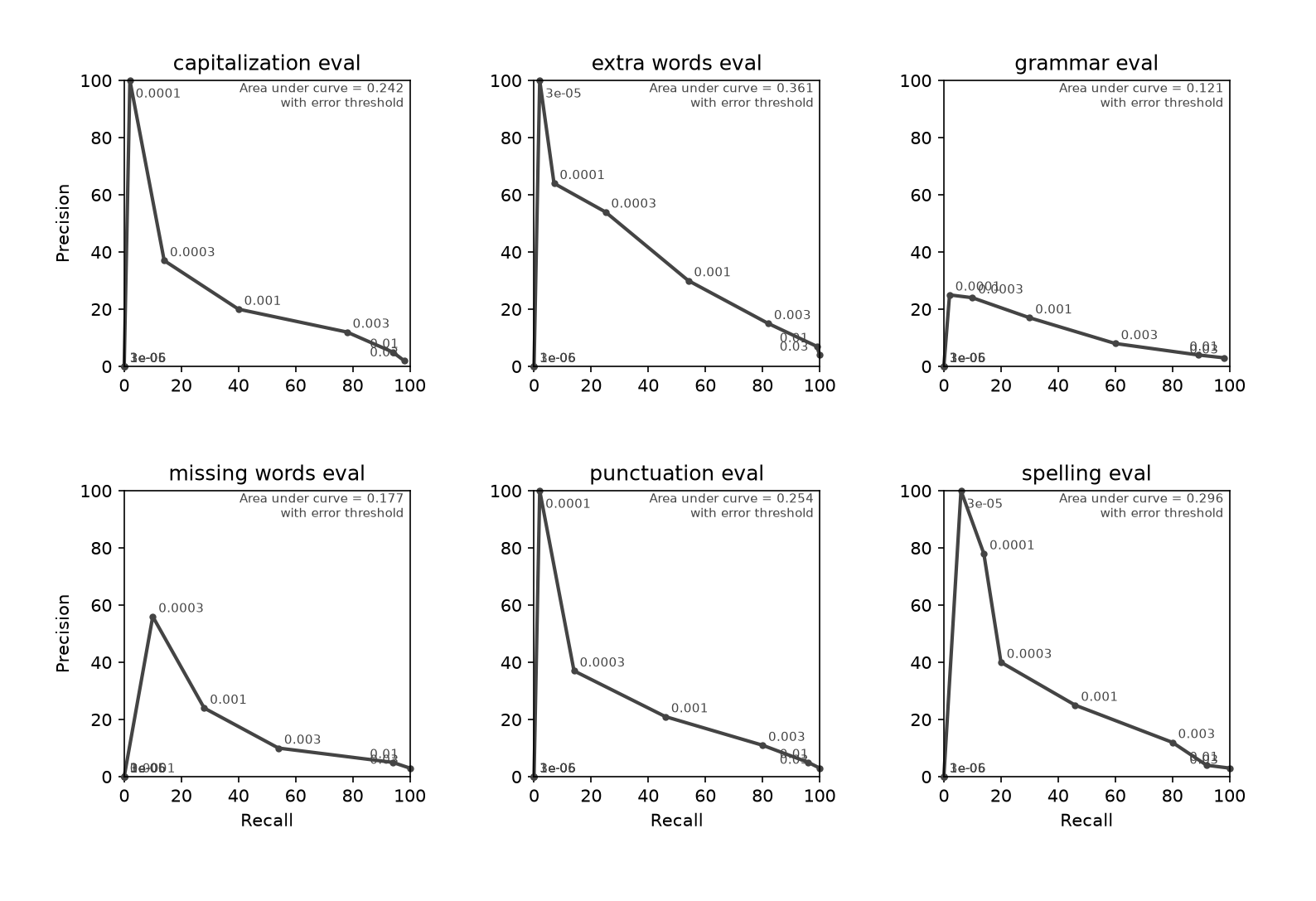
I had wanted this to work because it made so much sense to me. Letting all of the models participate in the vote feels egalitarian. More importantly, it is a typical approach in many machine learning methods. Geometric mean is a common way for ensemble models to vote. It usually takes the form of first taking the logarithm of the output of each model, then adding them together, but the end result is the same. But I can’t argue with the results. At least for the variants that I tried, it looks like the minimum combination rule is the winner.

Circling back to the min approach, because of the β parameter, it's actually quite conservative, so it’s not as fragile as most winner-take-all operations tend to be. Also, in a proofreading application, it’s not terrible to have some false alarms. The cost of a false positive is modest. So if it catches all of the errors (near perfect recall) but half of the words that it flags are actually correct, (50% precision) then that still a decent win. It gives the human a much shorter list of things to check before they can confidently share their writing.

Revisiting the minimum() compositing approach

Now that classic additive smoothing is implemented, it's worth a peek to see whether it helps out in the min-combination case.

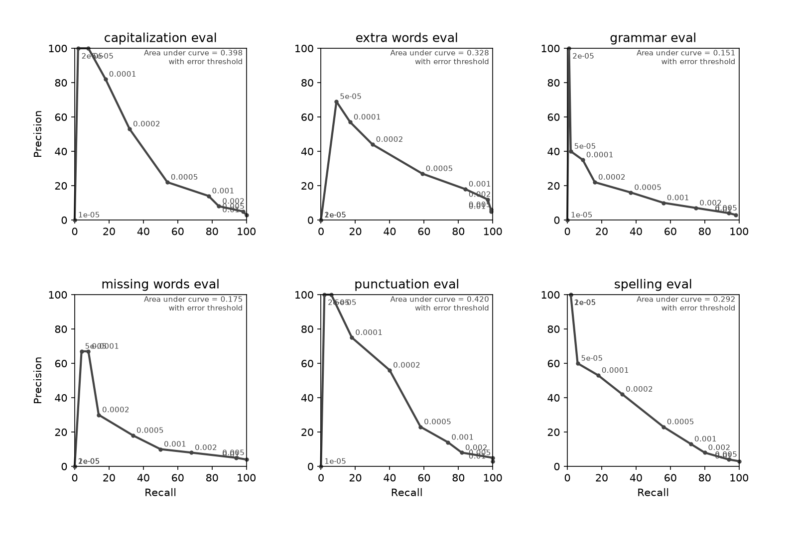
The results are promising. AUC for some of the evals is slightly up and for others slightly down. The highest one is 0.42, the highest found so far. It's notable that this is without doing any kind of a search across hyperparameters to find the best-performing combination. It's interesting enough to keep α around for some additional exploration.

Optimizing models one at a time

The ensemble model we're using here has gotten complex. There are several hyperparameters that can be traded off against each other: error threshold, α, β, and tokenizer alphabet size. And we still haven't investigated the possibility of adding other models into the mix. And to further stir the pot, there is no reason that every model in the ensemble should share the same error threshold, α, and β. The number of knobs to dial is multiplying and a strategy that rests on exhaustively trying every combination is not going to be feasible.

A useful way to approach this is to break the large optimization problem down into smaller, more tractable problems, and one way to achieve this is by optimizing models individually before adding them together. One thing we're missing before we can do this is a single optimization criterion, a number that we can try to make as high (or low) as possible. Ideally it's a number that reflects everything we care about in one place.

AUC is a reasonable step in this direction, because it combines precision and recall into a single value. Unfortunately, it doesn't go far enough because it is only defined across a range of values. It wouldn't help us choose a single error threshold. Also, I've conveniently papered over the fact that AUC values can only be meaningfully compared when the parameter being varied is the same (and at the same levels) in every plot. That isn't a constraint I've been respecting.

Optimizing for F_ρ

A better optimization criterion is the F-score. It's most common manifestation is the F₁:

F₁ = 2 × precision × recall /
       precision + recall

The product over the sum of precision and recall gives a single metric that balances the concerns of them both. When they are both scaled from zero to one (rather than expressed as a percentage), multiplying by 2 ensures that F₁ will also fall between 0 and 1, with larger being better.

Often in a particular application, recall is more important than precision or the other way around. There is another formulation of the F-score that allows us to put a finger on the scale.

F_ρ = (1 + ρ²) × precision × recall /
       ρ² × precision + recall

The factor ρ represents how much more important recall is than precision. For example, ρ = 2 indicates that recall is twice as important as precision, that is, that suffering two false positives is just as bad as a single false negative.

(F_ρ is usually presented as F_β, but since we're already using β for upward-biased additive smoothing that would have been confusing.)

As mentioned earlier, when using the minimum combination rule for ensemble models, precision of the combined models will tend to be lower than individual models and recall will tend to be higher, but the exact behavior here will depend on how much overlap there is between the errors detected by the two models. ρ = 1/2 is a good starting point, since a model's precision is more important to us than its recall, but ρ will remain a hyperparameter that we can adjust to influence the final performance.

Direction set methods: Optimizing one parameter at a time

The plots so far have shown precision and recall for varying values of a single parameter. This can be imagined as exploring a complicated world in one direction at a time. Viewing it this way gives a maddeningly narrow slice of what the countryside looks like. But now that we are up to four hyperparameters per individual Markov model (α, β, error threshold, and tokenizer alphabet size), we have scant hope of being able to visualize the complete landscape by any method.

Luckily, now that there is an optimization criterion defined we don't have to visualize the whole landscape. We're only interested in finding the highest point. This can be done by cycling through the directions available and traveling them one at a time, finding the highest point along one direction before moving on to the next. When we can cycle through all the directions without finding a higher point, we'll know we've arrived. This guarantees that we'll get to the top of the nearest hill, and we just have to hope that the hill we're on the knee of is the higihest one in the land.

Working with a set of directions (a direction set method) is a good way to navigate when it's not practical to calculate the gradient—when we can't read the slope of the ground and head uphill.

As a side note, this approach is the basis for Powell's method, although Powell's method makes the additional refinement of using prior search experience to choose a better exploration direction. Like most algorithmic refinements it makes the method more efficient for most problems, but it's possible to craft others that break it badly.

A tool for this job: Redsho

In 2019 I needed an optimizer that, like Powell's method, was gradient-free. I also wanted to make it tougher. Powell's method assumes that you're already somewhere on the hill you're trying to climb; it finds the local optimum. Most implementations also assume that the landscape it's traversing is smooth. If you've ever been outdoors, you know that these assumptions are frequently broken in the practice.

I built a direction set method that overcame these weaknesses, but at a cost. (There is always a cost! No lunch is free.) It requires a set of values to check in each direction, rather than exploring continuously. Another way of saying this is that it is a discrete optimizer, rather than a continuous optimizer. And it uses some random jumping to avoid getting stuck in ruts, but its jumps are heavily influenced by the best options it has discovered so far, similar to evolutionary algorithms.

This so-called Evolutionary Powell's method sat quietly collecting dust in a repository for a few years. Now its moment of usefulness has come! Of course with the benefit of seven more years of software engineering experience, I cringed at the devil-may-care quality of the project and felt compelled to give it a glow up before using it to tune Markov models. I'm glad I did. In the process of refactoring and adding type hints and tests I discovered several disturbing bugs and failure modes. It was broken in subtle ways, but now it's on more solid engineering foundations, and I feel more confident releasing it into the Python community.

This robust evolutionary direction set hyperparameter optimizer (Redsho) is now available on PyPI and in public repository services, including Codeberg and GitHub. It can be installed in any project with uv add redsho or pip install redsho. Detailed implementation instructions are in the repos' READMEs.

Tunable Markov Models

Armed with an optimizer, it was time to modify the first order Markov model to include a tuning step. After the model is trained by counting unigrams and bigrams in a collection of documents, it undergoes a second step where it uses redsho to explore values of α, β, and error threshold. This tuning step uses performance on the evaluation data set to calcaulate precision, recall, and F-scores. To be more precise, I assumed an error threshold of 1 and introduced a scaling factor. This sets it up so that multiple models all come out of the process scaled so that their best performance occurs with an error cutoff of 1.

An initial pass at tuning gives α = 2.15e-05, &beta = 0, and error threshold = 3.59e-05 for a forward model and α = 2.15, β = 10, and error threshold = 5.99e-05 for a backward model. Woohoo!

Next steps

We're right in the middle of this line of inquiry, but this post is already long, so I'm going to break it here and pick it up in the next post.

Building proofreaders

Now that there are tunable models, the next logical step is to put them into proofreaders and see how they perform. With any luck they will have higher recall and precision. I hope.

Adding more models

More importantly, with pre-tuned Markov models it becomes practical to combine more of them confidently. This opens the door to adding first-order models that skip words and second-order models into the basic forward-plus-backward model combination. This brings more information to bear on the proofreading decision and opens up the possibility of more sophisticated decisions. Hopefully this will start to make a dent in the grammar evals, which require the most context and where performance has been lagging the other evals.

Separate tuning and eval data

You may have noticed that I've double-dipped, using eval data for both tuning (validation) and evaluation (testing). That is a no-no because it can lead to artificially high evaluation scores. It's like allowing students to study the final exam questions before the exam. I'm going to need to build a separate data set, structured like the eval data, that is specifically for use in tuning.

Things are getting good!

If you are one of the three people still reading this post series, you probably noticed that this installment has a lot more side quests and dead ends than the others. This is a sign that we're getting to the juicy part. Striking out into the unmapped wilderland where there are no signposts. Charting our own course up the mountain means plenty of trial and error and trial again. I decided to include it, rather than paper over it and pretend that progress occurs in a straight line.