We're coming into this installment with some good momentum, but despite that (because of that?) it's a good time to pause for some house cleaning. The sparse first-order models and second-order models with size limits work so much faster and smaller than everything that came before, that the earlier work can be safely set aside. Those failed experiments are relegated to the git history and cleaned out of the code, as are all references to them.

Downsizing

This is a little painful. I was proud of getting the database models working. I thought I might be able to make a longer run with NumPy-backed models. But that's not what happened, and hanging on to all that code will just slow things down. Every extraneous line of code is a liability—something that might obscure the bug you're looking for or require updating or take extra time to test. The code is still in there if we ever need to retrieve it, but until then it will just be in the way. The artisanal approach is to generate and deprecate code with abandon. Kill your darlings.

Not only does this shrink the repository, but it also frees me up to make space on my hard drive. Some of the deprecated models, once trained, were enormous. 12 GB for the dense first-order models. I filled up my hard drive at several points during the last couple of posts and had to clean out discarded models. With the deprecation it allowed me to wipe all those from my disk and once again get some breathing room.

RAM has also been an ongoing issue. When training several models in succession, as part of running tests or evals, memory gets full to overflowing very quickly. I figured out that I have to take care and free up the memory used by each model when I'm done with it. This took some research and trial and error but I figured out that I could run clear() on each n-gram dictionary in the models to reclaim all their memory. Each model now has a delete() method that implements this. Now I can run models in succession with no issue.

Living small is part of the artisanal process. The constaints are not a barrier to the final product. They are an important shaping force that help it become what it needs to be. You can't come in at the end of a project and magically shrink it. Often the decisions made along the way are in direct opposition to that. You can only build small if you keep it small, working with what you've got as you go.

Refactoring

A rule of thumb that I have for myself is that the right time to refactor is right when you see it. Whether it's renaming a variable, pulling a reuasable snippet into a function, or pulling out a parent class from sibling classes, making the code clearer is always most helpful right now. This sparks of insight on how to clarify start to fade after a while, and you get used to the mental gymnastics of working with it as is, so I try to strike while the iron is hot.

In that spirit, the proofreader has evolved beyond science fiction. The larger Project Gutenberg training data sets now extend far beyond scifi, and it's likely that the training data set will grow futher still. It's still limited to the English language, so proofread-eng is now a better name for it than proofread-eng-scifi.

It's still a small-ish project and I like to stay as close to the code as I can get away with, so I don't use a full featured Integrated Development Environment (IDE) like VSCode or PyCharm. Instead I try to get by with the vim text editor and command line operations.

Making a wide ranging change like a package and repository name first requires figuring out everywhere the name exists. This command is helpful for that.

grep -r --include \*.py "proofread_eng_scifi" .

• grep finds things
• -r drills down into directories recursively
• --include \*.py only checks files whose names end in .py
• "proofread_eng_scifi" is the string to look for
• . signals to start looking in the current directory

It turns out that it occurs exclusively in import statements. Replacing it happens with this command.

sed -i '' -e 's/proofread_eng_scifi/proofread_eng/g' *.py

• sed (stream editor) is a command to modify text
• -i '' says not to create backups of the files before modification (living dangerously)
• -e instructs it to execute the command that follows
• 's/proofread_eng_scifi/proofread_eng/g' says to swap (s) the string proofread_eng_scifi for the string proofread_eng everywhere in the file, even if it occurs multiple times on the same line (g)
• *.py says to do this for all Python files in the directory.

I ran this separately in each directory containing files that needed renaming. There is certainly a way to automate this so that it changes all the .py files at once without descending into the .venv directories and possibly modifying those, but 2 minutes of twiddling wasn't enough to figure it out.

I changed the names of the repositories as well. Thankfully all three of the git hosting services I use (Codeberg, GitHub, GitLab) maintain the links to the old repository name and redirect them. I won't need to update any of the links in old posts. They'll all end up where they need to go.

New eval: Missing words

I've been in the habit of procrastinating eval work until the end of each post, but then it just sits there unused until I get to the next one. This time I'm more disciplined. I'm kicking off a new eval right away. A common prose failure mode is a missing word, but it's not one that's well represented in the evals yet. It feels worthy of its own category, especially since it is a particular type of error and may prove harder for some models to detect than others.

The performance on the missing words eval is similar in every important way to the other evals. Not interesting enough to throw up a plot at this point.

A first-order Markov model, but running backward

A cool thing about the proofreading problem is that we already have the complete text. There's not an implied relationship between token order and time. We can look forward just as easily as we can look back. It would be a shame to have the ability to see into the future and not use it.

It is a straightforward thing to flip the direction of a first-order model to make it run backward.

The forward version finds the conditional probability of a token pair, given the occurence of the first token.

P(AB|A) = count(AB) / count(A)

The backward version tweaks that by making it conditional on the occurrence of the second token.

P(AB|B) = count(AB) / count(B)

The necessary changes in the code are minimal. The difference between forward and backward first-order models is only a shift-by-one difference in the index of the token sequence, to pull out the second token in the pair instead of the first.

The behavior is similar too, but not identical. Looking at the forward and backward precision-recall lines side by side shows that some are clearly higher than others. On some evals the forward model performs better, but on other evals it's the other way around. This suggests that the two models are picking up on different patterns, which makes sense, given their different approaches. And as every comic book reader knows, when there are two heroes with different strengths you absolutely have to have ... *drumroll* ... A Teamup!

Combining forward and backward models

There are a lot of ways to combine the estimates of two models assessing the likelihood of a particular token appearing. Each will have its own likelihood estimate. The combined likelihood could be the maximum of the two, the minimum of the two, the average of the two, or any number of other schemes. Rather than brute force trying them all, it's helpful to develop some reasoning behind the choice.

The idea behind combining models is that each of them have different blind spots. If there is a sequence of tokens A, B, C, and we want to find the likelihood of B, then a forward first-order model will use the sequence AB to do that and a backward first-order model will use the sequence BC. It could be that B frequently follows A, so the likelihood of B given A is high. But it could also be that B rarely precedes C, so the likelihood of B given C is low. In this situation it makes sense to given every model veto power. Since the question the models are tasked with answering is "Is this token weird?", any single model detecting weirdness can answer that question with a yes. In this case, weirdness is a likelihood below the threshold set by the proofreader.

The math that goes along with this is the minimum operator. The likelihood of a particular token in a multi-model ensemble is the minimum of the likelihoods assigned by all the models in the ensemble.

Making models cautious

The downside of the frequentist method being used here is that it gets really wonky when there aren't many observations. If token A has been seen once but AB has not been seen, then P(AB | A) is 0/1 or 0. Assigning something a probability of zero is generally a bad idea. That suggests that it is impossible and that the universe will decay to heat death before it that event happens. This should be avoided in most sensible applications, a rule of thumb named Cromwell's Rule after Oliver Cromwell who authored the 17th century banger "I beseech you, in the bowels of Christ, think it possible that you may be mistaken." Today we rephrase that as "Never say never".

A common way to steer clear of zero probability estimates is additive smoothing, where a number called a pseudocount is added to the numerator and denominator. To implement this in a classic way, known as Laplace Smoothing, we would add 1 to AB and the dictionary size (e.g. 20,000) to A, so that even before any observations are made, the likelihood estimate of B given A is 1/20,000. It's small, but not zero. And, summed up over every possible two-token sequence starting with A, it adds to 1. If A always precedes B and the sequence AB is observed 20,000 times then the likelihood of B given A will be 20,000/40,000 or 1/2. No matter how many times the sequence AB is observed, the likelihood of AB will never reach one.

Additive smoothing is a step in the right direction, but here we want to go a step further than making the model approximately correct. We want it to err on the conservative side, to hold off from making a low-likelihood determination about a token until it has some experience under its belt and can make that declaration confidently. We want the estimate to be high, and then get lower with more observations, only crossing the threshold once the determination of weirdness can be made with confidence.

Upward biased additive smoothing

To get this effect, it's possible to add a pseudo-pseudocount to the likelihood estimate, adding the same constant to both the unigram and the bigram counts, to both the numerator and denominator. Traditionally, the constant used in additive smoothing is a Greek letter alpha. For this variation of additive smoothing, I'll use the Greek letter beta, β, for the constant.

The effect of this modification is to drive the likelihood estimate upward toward 1. In fact, before any observations are made, all likelihood estimates are (0 + 1)/(0 + 1) = 1/1 = 1. This is clearly nonsensical, estimating that every possible outcome is absolutely certain (think Everything Everywhere All at Once), but most importantly for error detection, it doesn't estimate anything to be at or near zero.

Imagine that the first time token A is encountered it is followed by B. The count of A is 1, the count of B is 1, and the likelihood of B given A is (1 + 1)/(1 + 1) = 2/2 = 1. Still high. Still OK for our purposes. At that point, the likelihood of C given A is (0 + 1)/(1 + 1) = 1/2. It's still not zero or even very small, which is exactly what we want. After all, A has only been seen once. How could the estimator possibly be confident about what should or shouldn't come next?

In order to get P(AB|A) down to 0.1, A would have to occur 9 times and never be followed by B. To get to 0.01, 99 times. For 0.001, 999 times. To get down to 1/n, A would have to been n-1 times without B following it. Adding in the βs forces the estimator to gather more experience before it can reach any low-likelihood estimates.

For β = 2, the number of times A has to be seen to reach a low estimate doubles. For 0.1, 18 times, etc. In general, for arbitrary β > 0, a likelihood of 1/n corresponds to β (n - 1) observations that do not include that outcome.

So how well does this grand idea work?

It works kind of OK. After some hunting around through dictionary sizes, error thresholds, and values for β, I found a combination that was good enough to be interesting.

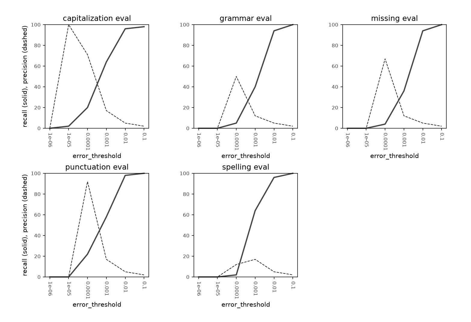
The reason I say it was OK, and not "good" is that precision is still low in some cases. The plan was to get several models with high precision and low recall, and combine their estimates with the minimum() function to get a composite model with medium-to-high precision and medium-to-high recall. Using a minimum rule for combining models will only ever drag precision down and lift recall up. For it to work we would need to start with high precision across the board. That's disappointing. It will require a change in the appoach.

Another thing to note about these plots is that they show performance curves with sharper peaks than we've seen before. This means that smaller changes in the parameters result in larger changes of tool performance, that performance is sensitive to hyperparameter values. The implication of this, combined with the fact that I just added a new hyperparameter to the mix, is that searching for optimally performing parameter combinations will require more trial and error. Possibly some automated hyperparameter optimization if it gets too tedious to do it my hand.

Looking at the backward first-order models the patterns are similar, but the performance seems to be a little better.

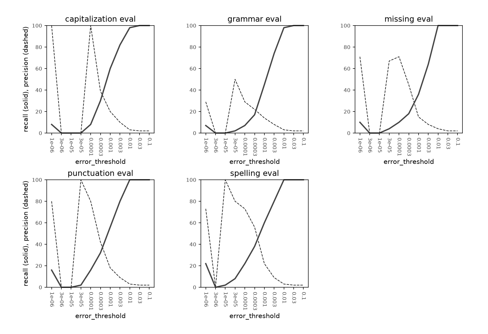
These plots are not quite the same, because I added twice as many error threshold points. They smear the performance peaks out a bit and give them more body. It's tough to tell whether the performance is really better or if the increased sampling density just gives a better picture of it.

Combining the forward and backward models and adding yet more error threshold evaluation points shows similar performance patterns. They are neither dramatically better nor worse than the individual models. These have been combined with the "minimum" method discussed earlier. It doesn't appear to have the powerful performance boost I hoped it would have, when coupled with biased additive smoothing.

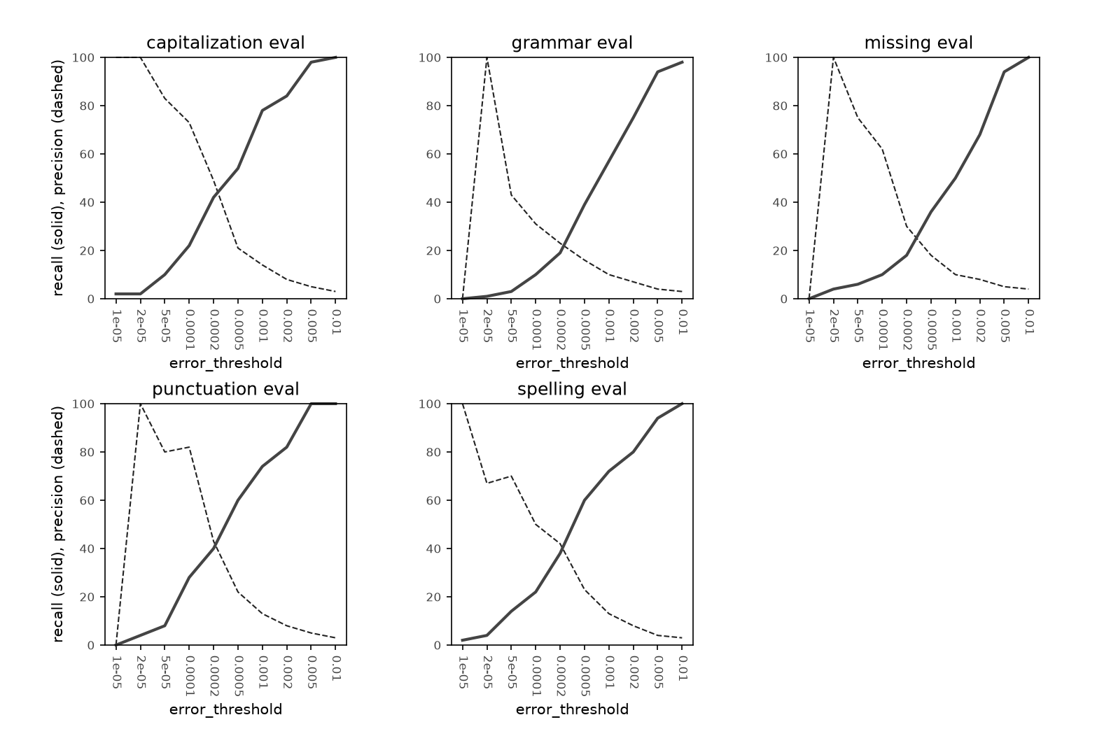
The forward/backward pair does show some promising performance on the evals where it the precision and recall curves cross over at around the 40% level, typically around 0.0002. But for grammar and missing words, for instance, that crossover still occurs at around the 25% level. The doesn't leave me with as much hope that we'll be able to add other models to the mix to get get recall, because that will only pull precision down more as long as I am using the minimum() function to combine them.

Next steps

This approach hasn't hit a wall, but it has hit a speedbump. The next order or business will be to search out another way to combine estimates from multiple models. We may have hit the limits of minimum().

We'll see how that goes before deciding what to do next. This work has hit the exciting phase were it is exploring new ground, and we can only see a step or two ahead at most.